
Intuition and Proof for Area Under a Polynomial
Intuition
Suppose you are timing a car with a stopwatch. It starts at rest and accelerates at a steady rate. At one minute, you clock it at a speed of 1 mile per minute. 30 seconds later, you clock it going 2.25 miles per minute. And another 30 seconds later, it is going 4 miles per minute (240 mph – it’s a very special car). Now you want to determine how much distance it crossed between minutes 1 and 2. If it was moving at a constant speed, this would be easy. For example, a car that travels 1 mile per minute for 10 minutes travels a total of 10 miles (10x1). When the speed is changing smoothly, it is more difficult to determine the total distance.
For simplicity, you could pretend that its speed changed in discrete steps. When you clocked it at 1 minute going 1 mile per minute, you assume it was going 1 mile per minute up until that moment. When you clocked it going 2.25 miles per minute at 1:30, you assume it was moving at that speed for the last 30 seconds. Finally, when you measured its speed as 4 miles per minute at minute 2, you assume that from 1:30-2:00, it was moving steadily at 4 miles per minute. What distance did it travel between minutes 1 and 2? 0.5 minutes × 2.25 miles per minutes + 0.5 minutes × 4 miles per minute = 3.125 miles.
Notice what we did here. We divided the time into even chunks of 30 seconds, measured the speed after each time chunk, and then assumed a constant speed for the duration of that time chunk: 0.5 minutes × speed1 + 0.5 minutes × speed2. And what is speed1 and speed2? Speed1 is the speed at the following time: 1 minute (start time) + 0.5 minutes (time chunk size) × 1 (chunk number) = 1:30. Speed2 is the speed at the time: 1 minute (start time) + 0.5 minutes (time chunk size) × 2 (chunk number) = 2:00. In general, the nth speed = the speed at (start_time + chunk_size × chunk_number). Let us call the time in minutes $t$, the speed at that time $f(t)$, the start time $a$, the end time $b$, the chunk size $\Delta$, and the chunk number $\lambda$. In that case, the $\lambda$th speed is $f(a + \Delta \cdot \lambda)$. To get an estimate of distance, we just need to multiply these speeds with the chunk size across the time interval from $a$ to $b$. Moreover, if we make the chunk size smaller, we will get a more accurate estimate because that will be the equivalent of measuring the speed more frequently during the 1 minute.
I’ve setup the problem so that the speed of the car is the square of the time (in minutes). Speed at minute 1 = 1 mile per minute, at minute 2 = 4 miles per minute. speed = $f(t) = t^2$. Graphically, the distance we are looking for is the “area under the curve” $x^2$ between $x=1$ and $x=2$. Notice the $\Delta$, which is the chunk size, is multiplied by the height of the function, which is the speed, to get the approximate area or distance for each chunk.
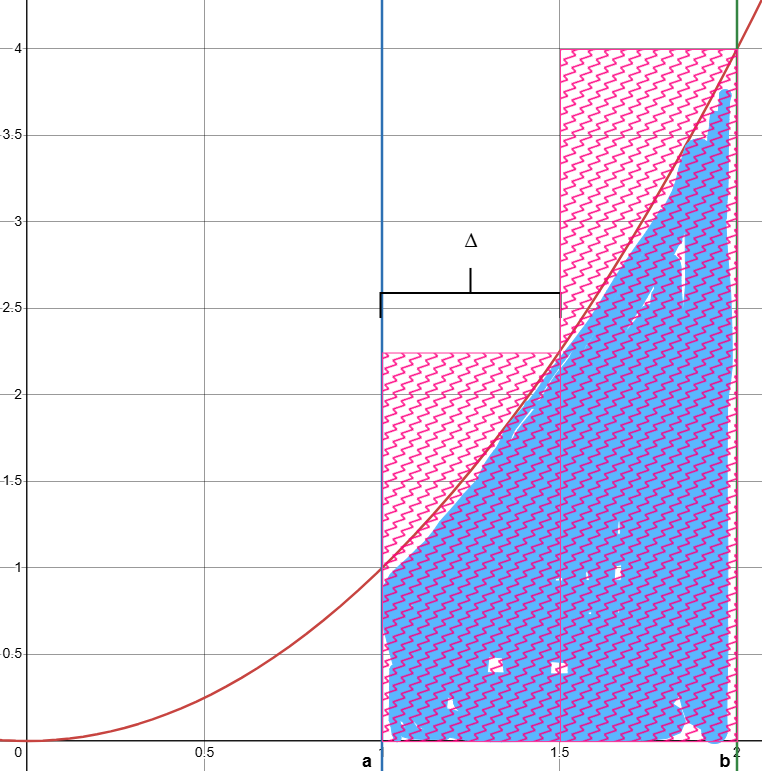
The red shows our overestimation of the distance, using 2.25 miles per minute for the first 30 seconds gives 2.25 × 0.5 minutes = 1.125 miles. And then 4 miles per minute for the second 30 seconds gives 4 miles × 0.5 minutes = 2 miles. This gives you a total of 3.125 miles, which we know to be too high, just as there is too much red overlaying the graph. We mentioned that we can get a better estimate if we reduce the chunk size.
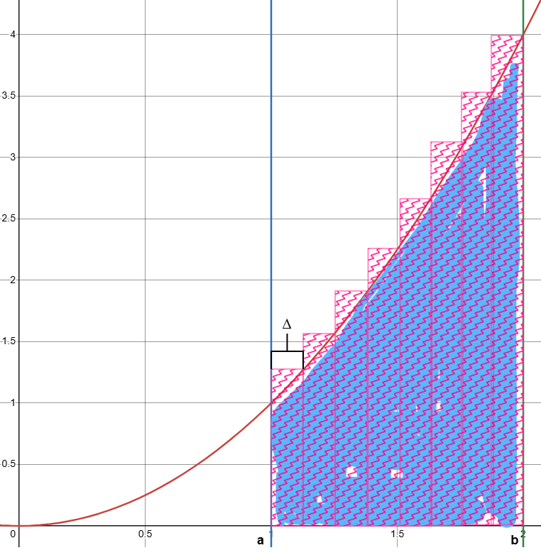
This is the equivalent of clocking the speed approximately every 7.5 seconds (0.125 minutes) and then calculating the distance by multiplying each speed by 0.125 minutes and summing it up. What if we kept making the chunks smaller and smaller?
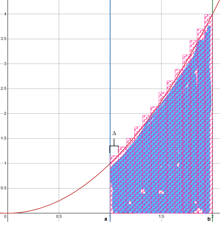
How beautiful! With just a bunch of plain rectangles, we can approximate the distance traveled really well, even though the speed of the car is constantly changing. I give thanks to God for such simplicity and beauty. And we can be filled with even greater wonder because our approximations can get better and better – to the point that they give us the exact answer. That should be impossible. Apparently, Math gives us wings to soar above the earth and ask the almost supernatural question: what would happen if the chunks were infinitely small and we added up infinitely many of them? How on earth could we know that? All we can say is, we can: Deo gratias! To get to this perfect solution, we must make $\Delta$ as small as possible.
Setting up the problem
The exact need described above, to reduce $\Delta$ and add the speed × time_chunks together can be represented mathematically in the following way:
\[\displaystyle \lim_{\Delta \to 0} \sum_{\lambda=1}^{(b-a)/\Delta} f(\lambda \Delta + a) \,\Delta = \lim_{\Delta \to 0} \sum_{\lambda=1}^{(b-a)/\Delta} (\lambda \Delta + a)^2 \,\Delta\]This is nothing fancy. We have the summation ($\Sigma$) of many chunks of size $\Delta$. How many chunks do we need? Enough to cover the interval from $a$ to $b$, so $(b-a)/\Delta$. Then we use the formula we derived above for speed_n = $f(\lambda \Delta + a)$ and multiply it by the small chunk size $\Delta$. Finally, we want to drive that $\Delta$ to 0, to make it as small as possible, and see if we can tell what happens as it gets smaller and smaller. This is indicated by $\lim_{\Delta \to 0}$. By the way, if you were not aware, the solution to this is exactly what is meant by the definite integral: $ \int_{a}^{b} x^{2} \, dx$.
The rest of this essay will be devoted to figuring this out. In some sense, it is already figured out approximately. You can plug in any small number into $\Delta$, like 0.001, and get a very good estimate. We wanted to know the distance traveled between minutes 1 and 2, so $a=1$ and $b=2$. If we set to $\Delta=0.001$, you will need to add up $(b-a)/\Delta = 1/0.001 = 1000$ terms. That might take you a while. We want to see if we can simplify this. It turns out we can – a lot. To do so, we will make use of three helpful formulas.
Formulas
-
nCr (“n choose r”) - how many combinations of r items can you make from n items?
\[\binom{n}{r} = \frac{n!}{r!(n-r)!}\] -
Binomial expansion - The expanded form of $(a+b)^n$ - For example, $(a+b)^2 = a^2 + 2ab + b^2$
\[(x + y)^n = \sum_{k=0}^{n} \binom{n}{k} x^{n-k} y^k\] -
Faulhaber’s formula - To sum the first n natural numbers raised to a power P, such as $1^3+2^3+3^3+4^3+…+100^3$
\[\sum_{k=1}^{n} k^{p} = \frac{1}{p+1} \sum_{j=0}^{p} \binom{p+1}{j} B_{j} \, n^{p+1-j}\]Here, $B_j$ refers to Bernoulli numbers, which are a sequence of numbers. The only one of interest to us will be the first one, $B_0=1$
Rather than solve our problem just for $x^2$, we will do it more generally for $x^P$ where $P$ is any positive integer. This will allow us to ascertain the definite integral or “area under the curve” of any polynomial.
With that, we have everything we need. Here we go!
Eliminate the Limit
We are attempting to determine what the summation (e.g. distance) approaches as $\Delta$ (e.g. time chunk size) approaches 0.
\[\displaystyle \lim_{\Delta \to 0} \sum_{\lambda=1}^{(b-a)/\Delta} (\lambda \Delta + a)^P \,\Delta\]($P$ is a positive integer.)
Note that this leaves a lot of terms. First of all, $(\lambda \Delta + a)^P$ will have $P+1$ terms (e.g. $(y+z)^3=y^3+3y^2 z + 3yz^2 + z^3$). And then we have one of those for every chunk, with the number of chunks approaching infinity!
Using binomial expansion, we can rewrite this as:
\[\displaystyle \lim_{\Delta \to 0} \sum_{\lambda=1}^{(b-a)/\Delta} \sum_{\beta=0}^{P} \Delta\, \binom{P}{\beta} (\lambda \Delta)^{P-\beta} a^\beta\]First, we swap the order of summation.
\[\displaystyle \lim_{\Delta \to 0} \sum_{\beta=0}^{P} \sum_{\lambda=1}^{(b-a)/\Delta} \Delta\, \binom{P}{\beta} (\lambda \Delta)^{P-\beta} a^\beta\]Then, we move out factors that do not depend upon $\lambda$ out of the inner summation.
\[\displaystyle \lim_{\Delta \to 0} \sum_{\beta=0}^{P} a^\beta \, \binom{P}{\beta} \Delta^{P-\beta+1} \sum_{\lambda=1}^{(b-a)/\Delta} \lambda^{P-\beta}\]We notice that the second summation can be rewritten using Faulhaber’s formula because it is the sum of a set of natural numbers starting at 1 raised to some power (for each inner summation, $P-\beta$ is a constant). After that, we’ll also move the $\Delta$ back to the right. This gives us:
\[\displaystyle \lim_{\Delta \to 0} \sum_{\beta=0}^{P} a^\beta \, \binom{P}{\beta} \frac{1}{P-\beta+1} \sum_{j=0}^{P-\beta} (-1)^j \binom{P-\beta+1}{j} B_j \frac{(b-a)^{P-\beta+1-j}}{\Delta^{P-\beta+1-j}} \Delta^{P-\beta+1}\]Admittedly, this seems way more complicated, and not a simplification! But this transformation is key. Originally we had $\sum_{\lambda=1}^{(b-a)/\Delta}$, which is the summation of infinite terms. Now, we have $\sum_{j=0}^{P-\beta}$, which is, at most, the summation of $P+1$ terms (merely 3 terms in our original example). Rather than summing infinitely many terms, we are summing just a few (${P+1}$) infinitely large terms containing $(b-a)^?/\Delta^?$. Additionally, since we moved the $\Delta$’s over to the right, they do something wonderful:
\[\displaystyle \lim_{\Delta \to 0} \sum_{\beta=0}^{P} \frac{a^\beta}{P-\beta+1} \, \binom{P}{\beta} \sum_{j=0}^{P-\beta} (-1)^j \binom{P-\beta+1}{j} B_j (b-a)^{P-\beta+1-j} \Delta^{j}\]Now, if $j=0$, $\Delta^j=1$, but if $j$ is anything else, $\Delta^j \to 0$ because $\Delta \to 0$. This $\Delta^j \to 0$ in the numerator multiplies itself with everything else and disappears. So every term except the one where $j=0$ vanishes!
\[\displaystyle \lim_{\Delta \to 0} \sum_{\beta=0}^{P} \frac{a^\beta}{P-\beta+1} \, \binom{P}{\beta} (-1)^0 \binom{P-\beta+1}{0} B_0 (b-a)^{P-\beta+1-0} \Delta^{0}\]Since $(-1)^0$, $\binom{P-\beta+1}{0}$, and $B_0$ are all equal to 1, this simplifies to:
\[\displaystyle \lim_{\Delta \to 0} \sum_{\beta=0}^{P} \frac{a^\beta}{P-\beta+1} \, \binom{P}{\beta} (b-a)^{P-\beta+1}\]$\Delta$ is no longer part of the expression! So nothing happens to this expression as $\Delta \to 0$, it stays exactly the same.
So, we are left with:
\[\displaystyle \displaylines { \int_{a}^{b} x^{2} \, dx = \\\\ \lim_{\Delta \to 0} \sum_{\lambda=1}^{(b-a)/\Delta} (\lambda \Delta + a)^P \,\Delta = \\\\ \sum_{\beta=0}^{P} \binom{P}{\beta} \frac{a^\beta (b-a)^{P-\beta+1}}{P-\beta+1} }\]If we pause to think about this, it is extraordinary. We started with an infinite problem: add together the “width” × “height” of an infinite number of infinitely narrow rectangles. We mere mortals could never do that. But now we have a solution that you could do by hand in a few minutes. Yes, I think we must pause there in awe…
Let us try it out on our initial problem, just for fun.
Brief Excursion - Try out the finite expression
In our initial problem, the accelerating car, $P=2$, $a=1$, $b=2$. Plugging that in, we get:
\[\displaystyle \displaylines { \sum_{\beta=0}^{2} \binom{2}{\beta} \frac{1^\beta (2-1)^{2-\beta+1}}{2-\beta+1} = \binom{2}{0} \frac{1}{2-0+1} + \binom{2}{1} \frac{1}{2-1+1} + \binom{2}{2} \frac{1}{2-2+1} =\\\\ \frac{1}{3}+\frac{2}{2}+1 = \frac{7}{3} }\]And that’s it! The car traveled exactly $2\frac{1}{3}$ miles between minutes 1 and 2. At this point, I feel inclined to move on to other Mirabilia Dei… but I can’t. Because I would like to see if we can eliminate the summation as well – that is – if there is greater simplification ahead. The expression as it stands has $P+1$ terms, which is very manageable. But if you are curious about how to reduce this further, buckle up!
Expanding and recombining $(b-a)^{P-\beta+1}$
As we’ve seen, we have a simple summation of $P+1$ terms now. However, if we do not yet plug in $a$ and $b$’s values and try to simplify it, $(b-a)^{P-\beta+1}$ expands in a larger number of terms. Using binomial expansion once again, we get:
\[\displaystyle \displaylines { \sum_{\beta=0}^{P} \binom{P}{\beta} \frac{a^\beta (b-a)^{P-\beta+1}}{P-\beta+1} = \\\\ \sum_{\beta=0}^{P} \binom{P}{\beta} \frac{a^\beta}{P-\beta+1} \sum_{k=0}^{P-\beta+1} \binom{P-\beta+1}{k}b^{P-\beta+1-k} (-a)^k }\]Combining the $a$ factors and separating out the $(-1)^k$, we get:
\[\displaystyle \sum_{\beta=0}^{P} \sum_{k=0}^{P-\beta+1} \frac{(-1)^k}{P-\beta+1} \binom{P}{\beta} \binom{P-\beta+1}{k} b^{P-\beta+1-k} (a)^{\beta+k}\]What does this mean? Each $\beta$ represents a polynomial of order $P-\beta+1$. The $k$ represents the terms within each polynomial. For example, if $P=2$, such as in our original example, this would expand as follows.
The first polynomial ($\beta=0$):
\[\displaystyle \frac{1}{3} b^{3} + \frac{-1}{3} 3 b^{2} a + \frac{1}{3} 3 b a^{2} + \frac{-1}{3} a^{3}\]The second polynomial ($\beta=1$):
\[\displaystyle \frac{1}{2} 2 b^{2}a + \frac{-1}{2} 2 \cdot 2 ba^{2} + \frac{1}{2} 2 a^3\]The third polynomial ($\beta=2$):
\[\displaystyle ba^{2} + -a^{3}\]This is what our present summation represents. But notice that we can sum them differently, as we would if we were simplifying this expression by hand, adding the polynomials above together. We would, for example, add up the coefficients of all the terms with $ba^2$, and then do the same for every other kind of term. If we simplified the expression in that way, we would end up with $P+2$ terms, but only the $\beta=0$ would have a non-zero coefficient for all $P+2$ terms. Let us call these terms, in the order that the summations give them to us: $\tau_0,…,\tau_{P+1}$. Let us call their coefficients $\delta_0,…,\delta_{P+1}$, where $\tau_t = \delta_t \cdot b^{(P+1-t)} \cdot a^{t}$.
For the example of $P=2$, the summation of the coefficients would be done vertically on the following table.
| $b^3$ | $b^2 a$ | $b a^2$ | $a^3$ |
|---|---|---|---|
| $1/3$ | $-1$ | $1$ | $-1/3$ |
| $1$ | $-2$ | $1$ | |
| $1$ | $-1$ |
Adding up the columns, we see that the result is $\frac{b^3}{3}-\frac{a^3}{3}$. But how do we get there in general? We need to rewrite our summation to be column-wise. We need it to sum the coefficients for each unique combination $b^?a^?$. So, eventually, the outer summation should be $\tau_0+\tau_1+..+\tau_{P+1}$, but we need a few steps to get there.
Let $t$ be the index of term $\tau_t$. The summation of each term involves more and more coefficients as $t$ increases, as seen in the table above.
For example,
- $t=0$ just includes the ($\beta=0$, $k=0$) term
- $t=1$ is the sum of the ($k=1$, $\beta=0$) term and the ($k=0$, $\beta=1$) term
- $t=2$ is the sum of the ($k=2$, $\beta=0$) term and the ($k=1$, $\beta=1$) term and the ($k=0$, $\beta=2$) term
As we see, $k+\beta=t$. So, with the goal of getting the outer summation to run across $t$ and the inner summation across $\beta$, we can first eliminate $k$, if we swap all $k$ with $[t-\beta]$. Because the second summation began at $k=0$ → $[t-\beta]=0$ → $t = \beta$ becomes the starting value. The summation goes to $k=P-\beta+1$ → $[t-\beta]=P-\beta+1$ → $t=P+1$. Therefore, we can rephrase the summation as follows:
\[\displaystyle \sum_{\beta=0}^{P} \sum_{t=\beta}^{P+1} \frac{(-1)^{t-\beta}}{P-\beta+1} \binom{P}{\beta} \binom{P-\beta+1}{t-\beta} b^{P-t+1} a^{t}\]This means that the $\beta=0$ involves the summation of all its $b^{P+1}a^0$, $b^{P}a^1$, …, $b^0 a^{P+1}$ terms, whereas $\beta=P$ involves only the summation of its $b a^{P}$ and $b^0 a^{P+1}$ terms. As mentioned earlier, now we would like to reorient the summation “column-wise”.
In our current summations, for each $\beta$, $t$ goes from that $\beta$ all the way to $P+1$. Notice that:
- When $\beta=0$, $t$ starts at 0. For all other $\beta$, $t$ cannot be 0.
- When $\beta=1$, $t$ starts at 1. For all other $\beta>1$, $t$ cannot be 1.
If we think about this backwards,
- When $t=0$, $\beta$ does not just start at 0, it can only be 0.
- When $t=1$, $\beta$, again, does not start at 1. It ends at 1. It can be 0 or 1.
With this in mind, we can write the summations. (Because $\beta$ only goes up to $P$, but $t$ goes up to $P+1$, we will separate out the $t=P+1$.)
\[\displaystyle \sum_{t=0}^{P} \sum_{\beta=0}^{t} \frac{(-1)^{t-\beta}}{P-\beta+1} \binom{P}{\beta} \binom{P-\beta+1}{t-\beta} b^{P-t+1} a^{t} + \sum_{\beta=0}^{t} \frac{(-1)^{P+1-\beta}}{P-\beta+1} \binom{P}{\beta} \binom{P-\beta+1}{P-\beta+1} b^{0} a^{P+1}\]If we also separate out $t=0$, we get:
\[\displaystyle \tau_0 = \frac{b^{P+1}}{P+1}\] \[\displaystyle \tau_1 + ... + \tau_P = \sum_{t=1}^{P} \sum_{\beta=0}^{t} \frac{(-1)^{t-\beta}}{P-\beta+1} \binom{P}{\beta} \binom{P-\beta+1}{t-\beta} b^{P-t+1} a^{t}\] \[\displaystyle \tau_{P+1} = \sum_{\beta=0}^{P} \frac{(-1)^{P-\beta+1}}{P-\beta+1} \binom{P}{\beta} a^{P+1}\]Our table above suggests that, somehow, $\tau_{m}=0$ (for all $m$, $1<=m<=P$) and $\tau_{P+1}=\frac{-a^2}{P+1}$. Why this works is not immediately obvious. Even in the table above, it seems odd that the columns $b^2a$ and $ba^2$ just happen to add up to $0$ and the $a^3$ column adds up to $-1/3$. Our next step is to see whether we can derive these results in general.
Simplify the middle terms
First, we know that, for any given $m$, $1<=m<=P$:
\[\displaystyle \tau_m = \sum_{\beta=0}^{m} \frac{(-1)^{m-\beta}}{P-\beta+1} \binom{P}{\beta} \binom{P-\beta+1}{m-\beta} b^{P-m+1} a^{m}\]Let us isolate and simplify its coefficient $\delta_m$ ($\tau_m$ = $\delta_m \cdot b^{P-m+1} a^{m}$). We begin by expanding the combination operators. It gets messier before it gets cleaner.
\[\displaylines { \delta_m = \sum_{\beta=0}^{m} \frac{(-1)^{m-\beta}}{P-\beta+1} \binom{P}{\beta} \binom{P-\beta+1}{m-\beta} \\\\ = \sum_{\beta=0}^{m} \frac{(-1)^{m-\beta}}{P-\beta+1} \frac{P!}{\beta!(P-\beta)!} \frac{(P-\beta+1)!}{(m-\beta)!(P-\beta+1-m+\beta)!} \\\\ = \sum_{\beta=0}^{m} (-1)^{m-\beta} \frac{(P-\beta+1)!}{P-\beta+1} \frac{1}{\beta!(m-\beta)!} \frac{P!}{(P-m+1)!}\frac{1}{(P-\beta)!} }\]A few things to note:
- $P-\beta+1$ in the denominator will cancel out the first factor of $(P-\beta+1)!$, making it $(P-\beta)!$, which gets cancelled out by the very last factor in the expression above.
- $(P-m+1)$ in the denominator can be rewritten as $(P-m+1)(P-m)!$. And now $\frac{P!}{(P-m)!}$ is almost $\binom{P}{m}$. We just need to multiply top and bottom by $m!$ and we will get $m!\binom{P}{m}$.
- If we move that extra $m!$ in the numerator over that $\beta!(m-\beta)!$ in the denominator, we get $\binom{m}{\beta}$. Putting this altogether, we get
Nifty!
The easy odd terms
To gain more intuition, let us expand the table above for the $P=3$ case (i.e. we are considering the infinite summation of the area under the curve $x^3$ between $x=a$ and $x=b$).
| $\tau_0$ | $\tau_1$ | $\tau_2$ | $\tau_3$ | $\tau_4$ |
|---|---|---|---|---|
| $b^4$ | $b^3 a$ | $b^2 a^2$ | $b a^3$ | $a^4$ |
| $1/4$ | $-1$ | $3/2$ | $-1$ | $1/4$ |
| $1$ | $-3$ | $3$ | $-1$ | |
| $3/2$ | $-3$ | $3/2$ | ||
| $1$ | $-1$ |
The odd terms, $\tau_1$ and $\tau_3$ follow a simple pattern. As you move in from the top and the bottom, the two cancel each other out by having opposite signs. We can discover this pattern mathematically to see how it occurs in general. Because $\tau_4$ ($\tau_{P+1}$) is a little different (it has one less row), we will analyze all the odd terms except the last term (which, in general, may be odd or even).
Recalling that $\beta$ represents the rows in the table above, we can see what happens when we add the first row and the last row ($\beta=0$ and $\beta=m$) or more generally the $i$th row from the top and bottom of the table ($\beta=i$ and $\beta=m-i$). We believe that they will be equal and opposite. Let us see. If we add the $\beta=i$ component of $\delta_m$ with its $\beta=m-i$ component, we get:
\[\displaylines { \frac{1}{P-m+1} \binom{P}{m} (-1)^{m-i} \binom{m}{i} + \frac{1}{P-m+1} \binom{P}{m} (-1)^{m-(m-i)} \binom{m}{m-i} \\\\ = \frac{1}{P-m+1} \binom{P}{m} \left( (-1)^{m-i} \binom{m}{i} + (-1)^{i} \binom{m}{m-i} \right) \\\\ = \frac{(-1)^{-i}}{P-m+1} \binom{P}{m} \left( (-1)^{m} \binom{m}{i} + (-1)^{2i} \binom{m}{m-i} \right) }\]Since $m$ is odd and $2i$ is even by definition,
\[= \frac{(-1)^{-i}}{P-m+1} \binom{P}{m} \left( -\binom{m}{i} + \binom{m}{m-i} \right)\]And since $\binom{m}{i} = \frac{m!}{i!(m-i)!}$ and $\binom{m}{m-i} = \frac{m!}{(m-i)!(m-(m-i)!)}$, they are equal. Therefore,
\[\delta_m = \frac{(-1)^{-i}}{P-m+1} \binom{P}{m} \left( -\binom{m}{i} + \binom{m}{m-i} \right) = 0\]Thus, $\tau_m = 0$ for all odd $m$.
The not-so-easy even terms
If you scroll up to the $P=3$ table above, $\tau_2$ also adds up to $0$ but in a less straightforward way: $\frac{3}{2} - 3 + \frac{3}{2} = 0$. How does this happen? First of all, we can’t use the simple idea of adding the $i$th element from the top and the bottom because, in this case, they will have the same sign.
When the nCr values are arranged in the form of a triangle (Pascal’s triangle), with each row number representing $n$, we notice that two elements of the row $n-1$ sum to a value in the row $n$.
 By Hersfold - Own work, Public Domain
We can show this mathematically.
The mathematics of Pascal’s triangle
We want to derive the entries in row $m$ of the triangle based on the entries in row $m-1$, where $m$ is even and so must be $>=2$. Assume $1<=\beta<=m-1$. If we add two adjacent entries in row $m-1$: \(\displaylines{ \binom{m-1}{\beta-1}+\binom{m-1}{\beta} \\\\ = \frac{(m-1)!}{(\beta-1)!(m-\beta)!} + \frac{(m-1)!}{\beta!(m-1-\beta)!} \\\\ = \frac{\beta}{\beta} \cdot \frac{(m-1)!}{(\beta-1)!(m-\beta)!} + \frac{(m-\beta)}{(m-\beta)} \cdot \frac{(m-1)!}{\beta!(m-\beta-1)!} \\\\ = \frac{\beta(m-1)! + (m-\beta)(m-1)!}{\beta!(m-\beta)!} \\\\ = \frac{m(m-1)!}{\beta!(m-\beta)!} \\\\ = \frac{m!}{\beta!(m-\beta)!} \\\\ = \binom{m}{\beta} }\)
Thus, for $m>=2$ and $1<=\beta<=m-1$, $\binom{m}{\beta} = \binom{m-1}{\beta-1}+\binom{m-1}{\beta}$.
Applying Pascal’s triangle to the even terms problem
So far we have:
\[\delta_m = \frac{1}{P-m+1} \binom{P}{m} \sum_{\beta=0}^{m} (-1)^{m-\beta} \binom{m}{\beta}\]But now we can apply the Pascal’s triangle rule to this for even $m$, by substituting $\binom{m}{\beta} = \binom{m-1}{\beta-1}+\binom{m-1}{\beta}$. However, our rule only applies for $1<=\beta<=m-1$, so we have to split off the $\beta=0$ and $\beta=m$ terms as well. The summation is in the middle.
\[\displaylines { \delta_m = \frac{1}{P-m+1} \binom{P}{m} + \frac{1}{P-m+1} \binom{P}{m} \sum_{\beta=1}^{m-1} (-1)^{m-\beta} \left( \binom{m-1}{\beta-1} + \binom{m-1}{\beta} \right) + \frac{1}{P-m+1} \binom{P}{m} }\]In expanded notation, we get
\[\displaylines { \delta_m = \frac{1}{P-m+1} \binom{P}{m} \left[1 -\left( \binom{m-1}{0} + \binom{m-1}{1} \right) + \left( \binom{m-1}{1} + \binom{m-1}{2} \right) -\left( \binom{m-1}{2} + \binom{m-1}{3} \right) +... -\left( \binom{m-1}{m-2} + \binom{m-1}{m-1} \right) + 1 \right] \\\\ = \frac{1}{P-m+1} \binom{P}{m} \left[1 -\binom{m-1}{0} -\binom{m-1}{1} + \binom{m-1}{1} + \binom{m-1}{2} -\binom{m-1}{2} -\binom{m-1}{3} +... -\binom{m-1}{m-2} -\binom{m-1}{m-1} + 1 \right] \\\\ = \frac{1}{P-m+1} \binom{P}{m} \left[1 -\binom{m-1}{0} + \left( -\binom{m-1}{1} + \binom{m-1}{1}\right) + \left(\binom{m-1}{2} -\binom{m-1}{2}\right) +... -\binom{m-1}{m-1} + 1 \right] \\\\ = \frac{1}{P-m+1} \binom{P}{m} \left[1 -1 + 0 + ... + 0 -1 + 1 \right] \\\\ = 0 }\]Therefore, even for even $m$, $\delta_m=0$, $\tau_m=0$.
The final term
Now, for anyone keeping score, we only have one term left to derive – the last column of our table, $\tau_{P+1}$. From what we derived earlier,
\[\displaystyle \tau_{P+1} = \sum_{\beta=0}^{P} \frac{(-1)^{P-\beta+1}}{P-\beta+1} \binom{P}{\beta} a^{P+1}\]With a few simple operations, we can simplify the coefficient $\delta_{P+1}$.
\[\displaylines { \delta_{P+1} = \sum_{\beta=0}^{P} \frac{(-1)^{P-\beta+1}}{P-\beta+1} \binom{P}{\beta} \\\\ = \sum_{\beta=0}^{P} \frac{(-1)^{P-\beta+1}}{P-\beta+1} \frac{P!}{\beta!(P-\beta)!} \\\\ = \sum_{\beta=0}^{P} (-1)^{P-\beta+1} \cdot \frac{1}{\beta!(P+1-\beta)(P-\beta)!} \cdot \frac{P!}{1} \\\\ = \sum_{\beta=0}^{P} (-1)^{P-\beta+1} \cdot \frac{(P+1)!}{(P+1)!} \cdot \frac{1}{\beta!(P+1-\beta)!} \cdot \frac{P!}{1} \\\\ = \sum_{\beta=0}^{P} (-1)^{P-\beta+1} \cdot \frac{(P+1)!}{\beta!(P+1-\beta)!} \cdot \frac{P!}{(P+1)!} \\\\ = \frac{1}{P+1}\sum_{\beta=0}^{P} (-1)^{P+1-\beta} \cdot \binom{P+1}{\beta} }\]Odd $P+1$
Notice that this looks similar to the simplified $\delta_m$. In fact, we already know that, for odd $m$, $\sum_{\beta=0}^{m} (-1)^{m-\beta} \binom{m}{\beta}=0$. Our current expression has almost the same form, if you replace $P+1$ with $m$ or some new variable. The one difference is that the summation stops at ${P}$ rather than at ${P+1}$. To make it match what we derived earlier, we will extend the summation by 1 and then substract it.
\[\displaylines { \delta_m = \frac{1}{P+1}\sum_{\beta=0}^{P+1} (-1)^{P+1-\beta} \cdot \binom{P+1}{\beta} - \frac{(-1)^{0} \cdot \binom{P+1}{P+1}}{P+1} \\\\ = 0 - \frac{1}{P+1} }\]This means that if $P+1$ is odd, $\tau_{P+1}$ = $-\frac{a^{P+1}}{P+1}$. You can see how this works in the $P=2$ table above. All the $\beta$ rows cancel each other out except for $\beta=0$, which, unlike in the odd $\tau_m$ terms, has no complement.
Even $P+1$
Now for when $P+1$ is even, which once again does not work out so easily, but it does follow the same pattern as our even terms approach above. If $P+1$ is even:
\[\displaylines { \delta_{P+1} = \frac{1}{P+1} \left[ (-1)^{P+1-0} + \sum{\beta=1}^{P} (-1)^{P+1-\beta} \binom{P+1}{\beta} \right] \\\\ = \frac{1}{P+1} \left[1 + -\left( \binom{P}{0}+\binom{P}{1} \right) + \left( \binom{P}{1}+\binom{P}{2} \right) -...-\left( \binom{P}{P-1}+\binom{P}{P} \right) \right] \\\\ = \frac{1}{P+1} \left[1 + -\binom{P}{0} + \left(-\binom{P}{1} + \binom{P}{1} \right) +...+ -\binom{P}{P} \right] \\\\ = \frac{1}{P+1} \left[1 - 1 + 0 + ... + 0 - 1 \right] \\\\ = \frac{1}{P+1} \cdot -1 }\]Therefore, for even $P+1$ as well, $\tau_{P+1}=-\frac{a^{P+1}}{P+1}$.
Conclusion
We began by trying to ask a question that, in a sense, shouldn’t be asked! How can we know the distance the car will travel between minutes 1 and 2 if the speed is increasing a tiny bit at every infinitesimal moment? But this is the beauty of mathematics. It would seem that God briefly permits us to step into the infinite, and there to make a few maneuvers, before having to return to earth. To solve a finitely bounded problem, we first made it infinitely complex. Then, we did a bunch of mathematical gymnastics to bring it down to finitude again, and we were satisfied with the solution. How curious!
To review our steps:
\[\displaylines{ \int_{a}^{b} x^{P} \, dx \\\\ = \lim_{\Delta \to 0} \sum_{\lambda=1}^{(b-a)/\Delta} (\lambda \Delta + a)^P \,\Delta \\\\ = \sum_{\beta=0}^{P} \binom{P}{\beta} \frac{a^\beta (b-a)^{P-\beta+1}}{P-\beta+1} \\\\ = \frac{b^{P+1}}{P+1} + \left[ \sum_{t=1}^{P} \sum_{\beta=0}^{t} \frac{(-1)^{t-\beta}}{P-\beta+1} \binom{P}{\beta} \binom{P-\beta+1}{t-\beta} b^{P-t+1} a^{t} \right] + \sum_{\beta=0}^{P} \frac{(-1)^{P-\beta+1}}{P-\beta+1} \binom{P}{\beta} a^{P+1} \\\\ = \frac{b^{P+1}}{P+1} - \frac{a^{P+1}}{P+1} \\\\ = \left.\frac{x^{P+1}}{P+1}\right|_{a}^{b} }\]May we never cease, for as long as we live, to be in amazement and gratitude and awe!